
This Excel tutorial shows you how to create pivot tables based on a dynamic named range that will expand as you add additional rows of data. This can be a huge time saver and helps to protect against inadvertent errors that result when pivot tables draw from only part of the data source.
Typically, when you build a pivot table, you select any cell in your data range and choose INSERT > Pivot Table.
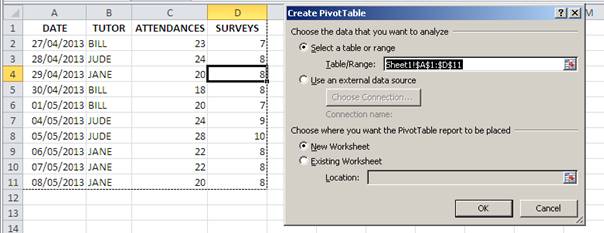
This generates the following dialogue box with a fixed Table/Range defined by an Absolute formula.
In the example illustration, that is: Sheet1!$A$1:$D$11
This is fine until you come to add more data.
Here is the same table with an additional week’s worth of course attendance data added. Refreshing the pivot table will not pull in the extra days data as the data range is still fixed.
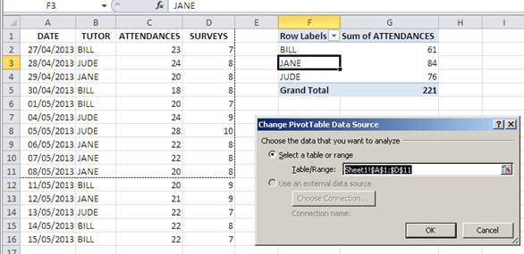
You can update this by clicking on the Pivot Table and then choosing Options > Change Data Source, but it’s an additional task to remember and if you have multiple pivot tables pulling from the same data range it is quite time consuming.
Using Named Ranges
Naming a range is relatively easy and when you use the name rather than the reference in a formula it really aids the understanding of the formula.
It’s fairly easy to do, just select the range and then type the name in the Name Box. Press enter and the name is defined. You can use the Name Box to select the named range as well.
Making the Named Range Dynamic with the Offset Formula
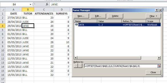
If we want to make our named range dynamic we can no longer work with the Name Box so we have to shift to the Name Manager. Formulas > Name Manager
As I’ve already set up a Named Range and imaginatively called it DATA, I can just amend the formula for this range. You could just as easily create a new name for your data range and then use the formula below:
=OFFSET(Sheet1!$A$1,0,0,COUNTA(Sheet1!$A:$A),4)
This is based on the powerful OFFSET function.
How does the OFFSET Function Work?
The OFFSET function returns a range based on a given starting point with a specified height and width (no of cells).
It’s a really useful formula for setting up dynamic ranges as you can vary the height and width on the result of another formula, in our example above this other formula is COUNTA which sets the height.
The OFFSET function has the following syntax:
= OFFSET(Starting or Reference Cell, Rows Down, Columns Right, Height, Width)
All of the inputs above can be number values (except the reference cell) or can refer to cell locations.
Here is a visual example to illustrate how the OFFSET function works
How the OFFSET function works
So the new dynamic range formula is:
=OFFSET(Sheet1!$A$1,0,0,COUNTA(Sheet1!$A:$A),4)
Which will start in the top left hand cell (A1), and then reference a range which is COUNTA(Sheet1!$A:$A) rows high and 4 columns wide. Which is just what we wanted.
Points to bear in mind:
It is good practice to start your source data with headers in cell A1, if you don’t you will have to amend your formula to reflect any extraneous rows before the data starts COUNTA counts all the non empty cells so you should also confirm that Column A doesn’t have empty cells, you could however refer to a different column if that held complete data Having set up the Dynamic range it is now time to adjust your pivot table so that it is now based on the new named range:
Select a cell in the pivot table
Options > Change Source Data
Overwrite the Range: with the name of your range, in my case DATA Click Ok and rest safe in the knowledge that your pivot will always look at the full range of data.